BENDULA ANIL KUMAR

In this article, we dive deep into the core concepts of multithreading. We will have a look at the profound understandings of the terms Concurrency and Parallelism with their description. Then, we compare the major differences between the two terms. Concurrency and Parallelism are often misunderstood to be somewhat similar but it is not the case when we consider it with aspects of Multithreading.

Concurrency

By Concurrency, we mean executing multiple tasks on the same core. In simpler terms, it relates to processing more than one task at the same time. It is a state in which multiple tasks start, run, and complete in overlapping time periods. An application capable of executing multiple tasks virtually at the same time is called a Concurrent application.

In case the computer only has one CPU or one Core the application may not make progress on more than one task at the exact same time. Instead, divide the time and the Core/CPU among various tasks. Concurrency is useful in decreasing the response time of the system.

Let us see this example and figure out the working of concurrent processes within a single core.

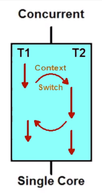
Here, we have two tasks T1 and T2 running on a single core. The task T1 is given a time slice for which it executes afterward the control of execution is given to T2 by the core this is called Context Switching, where a single core is shared among different processes or tasks effectively for small time slice to execute part of a process.

Parallelism

Parallelism is the ability of an application to split up its processes or tasks into smaller subtasks that are processed simultaneously or in parallel. It is the mechanism in which multiple processes execute independently of each other where each process acquires a separate core. This utilizes all the cores of the CPU or processor to run multiple tasks simultaneously.

Hence, to achieve parallelism the application must have more than one thread running on separate cores. In a single core CPU parallelism is not possible due to lack of hardware (Multi-Core Infrastructure). Parallelism is effective in improving the overall throughput resulting in faster execution. Let us look at an example:

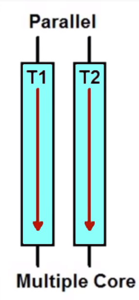
As you can see in the above figure, the two tasks T1 and T2 execute in parallel to each other. The two tasks run on separate cores and are independent of each other. This leads to faster execution because there is no time slice for the process. They do not have to wait for a process to finish and allocate CPU to other processes which were evident in the case of Concurrency.

Concurrency vs Parallelism

Now, we have a look at some key differences between Concurrency and Parallelism:

Concurrency	Parallelism
1. It is the mechanism to run multiple processes at the same time not necessary to be simultaneous.	1. It is the ability to split a heavyweight process into smaller independent subtasks and run those simultaneously.
2. Context Switching plays an important role in implementing concurrency.	2. In Parallelism, the sub-processes run separately so there is no overhead of Context Switching.
3. It is achieved using Single processing units or through a single core.	3. It requires Multiple Processing Units as processes run separately on different cores.
4. It runs on a single core so hardware is less required.	4. The implementation requires multiple cores for each of the processes so hardware cost is comparatively more here.
5. It increases the amount of work finished at a time and helps in decreasing response time considerably.	5. It is responsible for increasing the throughput of the system and in faster execution.
6. Concurrency is about dealing with a lot of things at once.	6. However, parallelism is about doing a lot of things at the same instant.

That’s it for the article, these core concepts are helpful in solving large scale problems. We looked into the description of each topic with their examples.

Feel free to leave your queries in the comment section below.

The post Concurrency vs Parallelism – Difference between Concurrency and Parallelism appeared first on The Crazy Programmer.

from The Crazy Programmer https://ift.tt/2Nzh6I4

In this article, we will understand the idea of Kadane’s Algorithm. We discuss this with the help of an example and also discuss a famous interview problem related to it. Then, we will look at the implementation and analyze the complexities of our approach.

Kadane’s Algorithm

This algorithm is useful in solving the famous ‘Maximum Sum Subarray’ problem. The problem states that given an array we need to find the contiguous subarray with maximum sum and print the maximum sum value. So, how does Kadane’s Algorithm help us in this problem?

The basic idea is to find all contiguous segments of an array whose sum will give us the maximum value. Kadane’s algorithm scans the given array from left to right. In the i^th step, it computes the subarray with the largest sum ending at i starting for each subarray.

For example, let us consider this array:

For the given array the maximum subarray exists for [ 1 2 3 6] highlighted in the image and the maximum sum is 12.

Algorithm

Now we look at the algorithm to find the maximum sum subarray.

1. We have two variables max_till_here and max_sum and initialize each variable with the first element of our array.

2. The max_till_here will hold the maximum of all elements or the maximum sum of all elements whichever is greater for a subarray. The max_sum will be our result variable which will contain the maximum of all max_till_here values.

3. So, we start iterating from index 1 or the second element of our array and keep doing the above steps. We keep adding the current array element if its sum with max_till_here is greater than the current element otherwise the max_till_here holds the value of the current element. We also update the max_sum variable with the maximum of max_sum and max_till here on each iteration.

Let us understand these steps with the above mentioned example:

Given Array arr : [ -4, 2, -5, 1, 2, 3, 6, -5, 1]

Initialize 
max_till_here = arr[0] or -4
max_sum = arr[0] or -4

For each iteration, we calculate max_till_here and max_sum as
max_till_here = max(arr[i], max_till_here+arr[i])
max_sum = max(max_sum, max_till_here)

We start at i=1, arr[1] = 2
max_till_here = max(2,-4+2) = max(2,-2) = 2
max_sum = max(-4,2) = 2

At i=2, arr[2] = -5
max_till_here = max(-5,2+(-5)) = max(-5,-3) = -3
max_sum = max(2,-3) = 2

At i=3, arr[3] = 1
max_till_here = max(1,-3+1) = max(1,-2) = 1
max_sum = max(2,1) = 2

At i=4, arr[4] = 2
max_till_here = max(2,1+2) = max(1,3) = 3
max_sum = max(2,3) = 3

At i=5, arr[5] = 3
max_till_here = max(3,3+3) = max(3,6) = 6
max_sum = max(3,6) = 6

At i=6, arr[6] = 6
max_till_here = max(6,6+6) = max(6,12) = 12
max_sum = max(6,12) = 12

At i=7, arr[7] = -5
max_till_here = max(-5,12+(-5)) = max(-5,7) = 7
max_sum = max(12,7) = 12

At i=8, arr[8] = 1
max_till_here = max(1,7+1) = max(1,8) = 8
max_sum = max(12,8) = 12

This is the working of the above algorithm for the above mentioned example in the image. You can see the max_sum obtained is 12.

Implementation in Java

Now we look at the implementation of the above discussed example in Java:

public class KadaneMaximumSumSubarray 
{
 
    static int maximumSubArraySum(int arr[])       //declaring method static help us to call method directly
    {
    int n=arr.length;
    int max_till_here = arr[0];                     //Initialize max_till_here and max_sum with 
    int max_sum = arr[0];                           // first element of array.
 
    for (int i = 1; i < n; i++)                     // We start iterating from second element.  
    {
        max_till_here = Math.max(arr[i], max_till_here + arr[i]);
        max_sum = Math.max(max_sum, max_till_here);
    }
    return max_sum;                             // At the end return max_sum which contain maximumSubArraySu
    }
 
    /* Driver Code to test above methods */
    public static void main(String[] args)
    {
    int arr[] = {-4, 2, -5, 1, 2, 3, 6, -5, 1};
    int max_sum = maximumSubArraySum(arr);             // we call the function to get the result 
    
    System.out.println("Maximum Sum of Contiguous Subarray is : "+ max_sum);
    
    }
}

Output:

Maximum Sum of Contiguous Subarray is : 12

Note: The above discussed approach also handles the case when the input array has all elements negative. In that case, the maximum element of array is our output.

Now, let us have a look at the time and space complexities of Kadane’s algorithm implementation in calculating the maximum subarray sum.

Time Complexity: We traverse the whole array only once while performing operations that require constant time so the time complexity is O(n).

Space Complexity: We do not use any auxiliary space so complexity is O(1).

That’s all for the article the algorithm is explained above you can try it out with other examples with the code.

Let us know if you have any queries in the comment section below.

The post Kadane’s Algorithm (Maximum Sum Subarray Problem) in Java appeared first on The Crazy Programmer.

from The Crazy Programmer https://ift.tt/3utRNrq

As we all know about HTML5 is the latest version of HTML currently available on the internet. HTML6 is soon to be released with some of the modified and new features and functionalities in it.

Here is a list of new tag attributes that can be comprised in HTML6 and will have namespace html, such as <html: html>, <html: head>, <html: title>, <html: meta>, <html: link>, <html: a>, <html: media>, <html: body>, and <html: button>, <form: form>, <form: input>, <form: select>, <form: status>, <form: label>, <form: submit>.

Image Source

<html: html>

It is equivalent to <html> tag for beginning of document.

<html: head>

Tag is similar to current <head> tag in HTML5.

<html: title>

It is also is similar to current <title> tag.

<html: meta>

In HTML6 metadata can be anything unlike HTML5. It is used to collect information for the developers.

<html: link>

It will be used to link external document similar to CSS. Current equivalent tag for this is <link> tag.

<html: a>

It will be used in place of anchor <a> tag in HTML6.

<html: button>

Tag is similar to <button> tag.

<html: body>

Similar to current <body> tag present in older versions of HTML.

<html: media>

Tag will include the tags such as <img>,<video>,<audio>. Instead of tag for each file type browser can easily know how to execute the above tags.

<form: form>

Tag will be used for creating new form and will contain the attributes method and action. Method can be POST or GET. Action would be for the destination of the data.

<form: input>

Tag will be used for taking input from the users. Here are the possible input types which can be included in HTML6.

• email
• text
• tel
• url
• number
• search
• datetime
• week
• month
• date
• time
• textarea
• datetime-local
• password
• file – (multiple)

The possible attributes on input are:

• name
• disabled
• readonly
• required
• autofocus
• placeholder
• novalidate

The following are attributes that will work on any input except file inputs:

• maxlength
• autocomplete
• spellcheck
• pattern
• match – New to HTML6.

<form: select>

Tag is for selecting the options and also similar to the current <input> tag. Here are some possible input types with suitable attributes.

• color
• select – (multiple)
• calendar – (range)
• meter – (range, step)

Attributes that work for all select types are:

• name
• required
• disabled
• readonly
• autofocus

<form: status> 

This will allow you to get status update or for the feedback purposes. This can be useful for upload progress bar. It will be similar to <progress> and <meter> in HTML5.

Attributes that will work for all status types are min, max, value.

<form: label> 

Tag can be used for labelling the input for the users.

<form: submit>

Tag will be used for submitting the input and is similar to <input type=”submit”> tag. Attributes that work for the <form: submit> tag are:

• value
• name

There are some more changes that can be included in the HTML6 for better compatibility and user experience. Given below are some of them:

• HTML6 dedicated libraries
• Freedom to Resize image
• Express Tags
• Annotations for images and videos
• Authentication Enhancement
• Better contact Information
• Pluggable languages
• Pluggable pre-processors
• Camera Integration
• Stronger micro-formats

HTML6 Dedicated Libraries 

For libraries that are very large requires a lot of issues and for this a cacheable version of libraries can be introduced in HTML6 for the ease of using and loading other libraries.

Freedom to Resize image

For better viewing experience and new tag <srcset> can be introduced in this version. In this browser can be able to resize and adjust the image according to window size and device resolution.  

Express Tags

<logo> </logo> for the logo on the page, <sidebar> </sidebar>, <navigation> </navigation> are some express tags.

Annotations for Images and Videos

In HTML5 we can annotate words but not images and videos but in this version annotations for videos and images also can be included. 

Authentication Enhancement

Although HTML5 was good in terms of security and authentication but for more better security keys can be stored off-site as to prevent people from gaining access. Therefore it can also be accepted by WHATWG.

Better Contact Information

Sometimes for pulling out our contact number, email we have to cut and paste it. A better contact information system can be included in this version.

Pluggable Languages

Effective and pluggable languages would be included in this version so that developers would be able to create a unique design within time and the browser would be able to easily implement this feature within a few steps.

Pluggable Preprocessors

Pre-processors are also present in the current HTML version. But in the new version, it would be optimized and will open a new window for developers.

Camera Integration

We generally use cameras and microphones for interacting with people. HTML6  would help us to access our media located in our device and we will get better control of the microphone and camera.

Stronger Micro-formats

There are some tags in HTML such as footer, paragraph, headline but it would be more efficient if standard web page sections are included such as address or phone number. It would boost the speed and quality of website.

Conclusion

There is no perfect language exist and there is always a chance of improvement. There is no official news yet but HTML6 will soon be released in the market and will be available for users. Hopefully, it will be better and easier to use than older versions.

The post HTML6 – New Features Expected and Release Date appeared first on The Crazy Programmer.

from The Crazy Programmer https://ift.tt/3sjQ2Ln

In this article we have a look at another interesting problem related to binary tree. Given a binary tree we have to invert the tree and print it. We discuss different approaches to solve this problem along with their time and space complexities

The inversion of a binary tree or the invert of a binary tree means to convert the tree into it’s Mirror image. In simple terms, it is a tree whose left children and right children of all non-leaf nodes are swapped.

Note: The leaf nodes will also get interchanged. It is recommended to learn In-Order and Post Order traversal before proceeding with this problem.

Let us look at an example of a binary tree:

 

In the above figure we see the sample tree and it’s inverted or mirror version.

Input:             20                                                  
                /       \
               /         \
              10          30                      
            /   \        /   \
           /     \      /     \
          5      15    25      35                


Output:            20                                                  
                /       \
               /         \
              30          10                      
            /   \        /   \
           /     \      /     \
          35      25   5      15

Approach 1 (Recursive Approach)

Follow these steps:

• We basically do a Post-Order Traversal of our tree starting from the root where we traverse for the left subtree first and then the right subtree before processing the root.
• At time of processing the root of each node we swap their left and right child respectively if their children are not null.
• We also check if the given root of binary tree is null or not. Then, we continue traversing for the left and right subtrees accordingly. If, we are at a leaf node it does not have any children for which we return null indicating that no swapping is required.
• To verify the tree is inverted or not we do the In-Order traversal of tree before executing the function and again print the In-Order traversal after doing inversion. You can verify the output using any traversal algorithm.

Now, let’s look at the implementation of above in code:

//Class containing attributes of each node of tree
class Node 
{ 
    int data; 
    Node left, right; 
  
    Node(int data) 
    { 
        this.data = data; 
        left = null;
        right = null; 
    } 
} 
  
class Tree 
{ 
    Node root; 
  
    void invertTree(Node node) 
    { 
        if (node == null) 
            return; 
  
        //we call or recur for left subtrees then the right subtrees
        invertTree(node.left); 
        invertTree(node.right); 
  
        //swap the left and right child of each non-leaf node*/
        Node temp=node.left;
        node.left = node.right; 
        node.right = temp; 
  
    } 
  
  
    /* Helper function to test invertTree() by printing In-Order traversal*/
    void printInOrder(Node node) 
    { 
        if (node == null) 
            return; 
  
        printInOrder(node.left); 
        
        System.out.print(node.data + " "); 
  
        printInOrder(node.right); 
    } 
  
    /*Driver code to test for sample tree*/
    public static void main(String args[]) 
    { 
        /* creating a binary tree and entering the nodes */
        Tree tree = new Tree(); 
        tree.root = new Node(20); 
        tree.root.left = new Node(10); 
        tree.root.left.left = new Node(5); 
        tree.root.left.right = new Node(15); 
        tree.root.right = new Node(30);
        tree.root.right.left = new Node(25);
        tree.root.right.right = new Node(35);
  
        /* print inorder traversal of the input tree */
        System.out.println("Inorder traversal of Input Tree is :"); 
        tree.printInOrder(tree.root); 
        System.out.println();
        
        
        System.out.println(); 
        /* convert tree to its mirror */
        tree.invertTree(tree.root); 
  
        /* Inorder traversal of the Inverted Binary tree */
        System.out.println("Inorder traversal of Inverted Tree is : "); 
        tree.printInOrder(tree.root); 
  
    } 
}

Output:

Inorder traversal of Input Tree is :
5 10 15 20 25 30 35 

Inorder traversal of Inverted Tree is : 
35 30 25 20 15 10 5

You can see the difference in output. The In-Order traversal for the given input tree displays output in sorted order and the In-order traversal of the Inverted tree gives output in reverse sorted order.

Time Complexity: We just traverse all the nodes present in tree so the time complexity will be O(n).

Space Complexity: If we consider the system stack space for each recursive call then complexity is O(n) otherwise it is O(1).

Approach 2 (Iterative Approach)

The main idea is to do a Level Order Traversal of the tree using a Queue. We enqueue the root first into the Queue. While we traverse all the nodes at a particular level we swap the left child and right child of each node. After this, we add the left and right child child of the current node into our queue to continue the level order traversal.

Finally, we print the In-order traversal of the tree to verify the inverted tree.

Let us have a look at the implementation:

// import the Queue interface of Collections implemented using Linked List
import java.util.Queue;
import java.util.LinkedList;
//Class for each node of tree
class Node 
{ 
    int data; 
    Node left, right; 
  
    Node(int data) 
    { 
        this.data = data; 
        left = null;
        right = null; 
    } 
} 
  
class Tree 
{ 
    Node root; 
  
    void invertTreeIterative(Node root) 
    { 
        if (root == null) 
        return; 
  
        Queue<Node> queue = new LinkedList<>(); 
        //Add root first
        queue.add(root); 
      
        //We do level order traversal 
        while (queue.size() > 0) 
        { 
            // Get node of each level 
            Node curr = queue.poll();
      
            // swap left child with right child 
            Node temp = curr.left; 
            curr.left = curr.right; 
            curr.right = temp;; 
      
            // enqueue left and right child 
            if (curr.left != null) 
                queue.add(curr.left); 
            if (curr.right != null) 
                queue.add(curr.right); 
        } 
      
    } 
  
    /* Helper function to test invertTree() by printing In-Order traversal*/
    void printInOrder(Node node) 
    { 
        if (node == null) 
            return; 
  
        printInOrder(node.left); 
        
        System.out.print(node.data + " "); 
  
        printInOrder(node.right); 
    } 
  
    /*Driver code to test for sample tree*/
    public static void main(String args[]) 
    { 
        /* creating a binary tree and entering the nodes */
        Tree tree = new Tree(); 
        tree.root = new Node(20); 
        tree.root.left = new Node(10); 
        tree.root.left.left = new Node(5); 
        tree.root.left.right = new Node(15); 
        tree.root.right = new Node(30);
        tree.root.right.left = new Node(25);
        tree.root.right.right = new Node(35);
  
        /* print inorder traversal of the input tree */
        System.out.println("Inorder traversal of Input Tree is :"); 
        tree.printInOrder(tree.root); 
        System.out.println();
        
        
        System.out.println(); 
        
        /* convert tree to its mirror */
        tree.invertTreeIterative(tree.root); 
  
        /* Inorder traversal of the Inverted Binary tree */
        System.out.println("Inorder traversal of Inverted Tree is : "); 
        tree.printInOrder(tree.root); 
  
    } 
}

Output:

Inorder traversal of Input Tree is :
5 10 15 20 25 30 35 

Inorder traversal of Inverted Tree is : 
35 30 25 20 15 10 5

Time Complexity: It is same as recursive approach which require O(n) time as we traverse all nodes of tree.

Space Complexity: We use a Queue which stores all the nodes during execution so complexity is O(n).

That’s it for the article you can try and execute the above code. Feel free to ask your queries in the comment section.

The post Invert a Binary Tree – Recursive and Iterative Approach in Java appeared first on The Crazy Programmer.

from The Crazy Programmer https://ift.tt/3bjaTaI

In this article we will learn how to design a LRU Cache, understand it’s cache replacement algorithm. We also look at description of LRU Cache with some examples. Then, we look at the implementation of this design in code with their complexity analysis.

Caching is a method of organizing data in a faster memory, usually RAM to serve future requests of same data in a efficient way. It avoids repetitive main memory access by storing frequently accessed data in cache. However, the Cache size is usually not big enough to store large data sets compared to main memory. So, there is a need for cache eviction when it becomes full. There are many algorithms to implement cache eviction. LRU caching is a commonly used cache replacement algorithm.

Least Recently Used (LRU) Cache organizes data according to their usage, allowing us to identify which data item hasn’t been used for the longest amount of time. The main idea is to evict the oldest data or the least recently used from the cache to accommodate more data followed with replacement of data if already present in the cache (Cache Hit) and bring it in the front or top of the cache for quick access.

Example:

Let’s consider a cache of capacity 4 with elements already present as:

Elements are added in order 1,2,3 and 4. Suppose we need to cache or add another element 5 into our cache, so after adding 5 following LRU Caching the cache looks like this:

So, element 5 is at the top of the cache. Element 2 is the least recently used or the oldest data in cache. Now if we want to access element 2 again from the cache. The cache becomes:

So, element 2 comes to the top of the cache. Element 3 is the least recent used data and next in line for eviction.

LRU Cache Implementation

We follow these steps to implement a LRU Cache in our program:

• We use two Data Structures a Deque or Doubly Ended Queue, where insertion and deletion can take place from both ends and a Hash-Map. The Deque will act as our Cache.
• In Queue, we enter each element at first/front of the queue, so we use a Deque. If we need to access any element already present in our cache we search that element in queue, remove it and then add it to the front of the queue/cache. But searching an element in queue could take O(n) time in worst case and will be a costly operation.
• So, to avoid this we use a Hash-Map which provides look-up or search time for our keys in O(1) time. Then, we can directly delete the element without the need to search in cache. So if our Hash-Map contains the data then we can just bring that element to the front of queue and add data as entry to our map for future look-ups.
• If our capacity is full then we remove from the rear end of Deque which contains least recent data. Along with this, we remove the entry of the element from our Map.
• So, we mainly need to implement two methods for our cache: One to get element from cache and other to add element into our cache following the LRU algorithm and above steps.
• In get method we need to just get the value of data item if it’s present in our cache. In put method we add the data into our cache and the Map and update the order of cache elements.

Why Hash-Map not Hash-Set?

Since we only need to search whether an element is present in our cache or not we can also do it by using a Hash-Set then what is the purpose of Hash-Map. The reason is while accessing resources from the Cache a key is required to access the data. The key will be unique for each data. So with the key we can access the actual data. In real life scenario, for a product there can be many attributes we need to access with the product key. As we know, Hash-Map stores data in Key-Value Pair the Key Field holds the key of data and Value field can hold the actual data or attributes.

Now let’s look at the implementation of above in Java:

//import the required collection classes
import java.util.Deque;
import java.util.HashMap;
import java.util.LinkedList;
import java.util.Map;

class CacheObject 
{
  int key;              // key to access actual data
  String value;         // data to be accessed by cache
  
  CacheObject(int key, String value) {
    this.key = key;
    this.value = value;
  }
}

public class LRUCache {
  
  //  queue which acts as Cache to store data.
  static Deque<Integer> q = new LinkedList<>(); 
  
  // Map to store key value pair of data items.
  static Map<Integer, CacheObject> map = new HashMap<>();
  int CACHE_CAPACITY = 4;

  public String getElementFromCache(int key) // get data from cache if key is already present.
  {
      
    // if item present in cache remove and add to front of cache
    if(map.containsKey(key)) 
    {
      CacheObject current = map.get(key);
      q.remove(current.key);
      q.addFirst(current.key);
      return current.value;
    } 
    
    return "No such element present in Cache";
  }
  
  public void putElementInCache(int key, String value) 
  {
    if(map.containsKey(key)) 
    {
      CacheObject curr = map.get(key);     // we check if element already present in cache through Map
      q.remove(curr.key);                  // remove if already present
    }
    else 
    {
      if(q.size() == CACHE_CAPACITY) 
      {
        int temp = q.removeLast();  // if cache size is full we remove from last of queue
        map.remove(temp);
      }
    }

    // then we just add already present item or new item with given key and value.
    
    CacheObject newItem = new CacheObject(key, value);
    q.addFirst(newItem.key);   
    map.put(key, newItem);
  }
  
  // Driver Code to test above methods.
  public static void main(String[] args) 
  {
    
    LRUCache cache = new LRUCache();
    cache.putElementInCache(1, "Product-A-Name");
    cache.putElementInCache(2, "Product-B-Name");
    cache.putElementInCache(3, "Product-C-Name");
    cache.putElementInCache(4, "Product-D-Name");
    
    // We get 2 from cache
    System.out.println(cache.getElementFromCache(2));
    System.out.println();
    
    // We print our queue and see 2 will be at front of cache    
    System.out.println(q);
    System.out.println();
    
    //Element 5 is not present in Cache
    System.out.println(cache.getElementFromCache(5));
    cache.putElementInCache(5,"Product-E-Name");
    System.out.println();
    
    //Now after adding 5 in cache it will be at front and 1 is deleted.
    System.out.println(q);
    System.out.println();
    
  }

}

Output:

Product-B-Name

[2, 4, 3, 1]

No such element present in Cache

[5, 2, 4, 3]

So this was the implementation of LRU Cache in code let’s have a look at the time and space complexities of our approach.

Time Complexity: Basically we implement this cache in O(1) time, as the search for an element present in cache require constant time and with our Map the search time is also constant. In put method, we add elements to front of cache which also require constant time. So overall time is O(1).

Space Complexity: We use a Deque which store n number of keys and a Map which store n Key-Value pairs so the overall space complexity is O(n).

That’s it for the article you can post your doubts in the comment section below.

The post LRU Cache – Design and Implementation in Java appeared first on The Crazy Programmer.

from The Crazy Programmer https://ift.tt/2Nr5HKb

In this article we look into the difference between Primary Key and Unique Key Constraints. We will see the description of both along with how to define a schema and create attributes in a table with these constraints.

Primary Key

A Primary Key is a key attribute or a column which is used to uniquely identify a row (tuple) in a table (relation). It maintains the integrity constraints of a table. A table can have only one primary key attribute. The data of primary key must be unique. Hence, no duplicate values are valid. Also, no NULL (empty) values are allowed during insertion as it violates the integrity constraint. The database automatically creates a Clustered Index over primary key which orders data on the basis of primary key.

We define a Primary Key Attribute as follows:

Column_Name DataType PRIMARY KEY

Unique Key

A Unique Key is a constraint or key attribute which also uniquely identifies a row in a table. It’s purpose is somewhat same as primary key. It differs in ways such as a table can have one or more than one Unique keys. It allows the possibility of NULL value insertion limited to only one null value insertion. In other words, Unique Key Constraints allow a column to have only one NULL value. No duplicate values are permitted. By default, the Unique key are generated in a Non-Clustered Index.

We define a Unique Key Attribute as follows while creating a table:

Column_Name Datatype UNIQUE

Now let us look at an example of creating a table with these constraints:

CREATE TABLE CARS
(
Car_Id INT PRIMARY KEY,
Car_Brand VARCHAR(10),
Car_NumberPlate VARCHAR(10) UNIQUE
);

Here Car_Id is the Primary key and Car_NumberPlate is the Unique Key of table CARS.

Let us assume we have these records in table CARS:

If we add a record like this:

INSERT INTO CARS VALUES(3,'Hyundai','');

This will add the record successfully since the unique key Car_NumberPlate allows one null value and show contents of database:

If we add any duplicate value in Primary key field Car_Id, it will show us error

INSERT INTO CARS VALUES(3,'Honda','TN056789');

So, when we try entering duplicate values to our Primary key Car_Id it shows the Unique constraint of the field is violated.

Also Read: Difference between Primary Key and Foreign Key

Difference between Primary Key and Unique Key

Now let’s look at the key differences between them:

Primary Key	Unique Key
1. It is the SQL constraint to uniquely identify rows of a table.	1. It is a unique identifier for rows when primary key is not present.
2. Primary Key does not allow NULL value insertion.	2. It allows one NULL value insertion.
3. Only one Primary Key can be present in a table.	3.There can be one or more than one Unique keys in a table.
4.  The main purpose is to enforce entity integrity.	4. The main purpose is to enforce uniqueness of entity data.
5. By default, the primary key column has Unique Clustered Index.	5. The unique key column has Non-Clustered Index.
6. It is useful in creating relationships between other tables.	6. It is useful for Data Validation.

That’s all for the article you can create a table like the example mentioned above, add some records and see it in working!

Feel free to ask your doubts in the comments section.

The post Difference between Primary Key and Unique Key appeared first on The Crazy Programmer.

from The Crazy Programmer https://ift.tt/2ZwG0KI

In this article, we see how to print the bottom view of Binary Tree. We discuss our approach to solve this problem and analyze the time and space complexities.

It is recommended to first learn Top View Of Binary Tree before proceeding with this problem. A lot of the implementation is based on the Top View Approach.

By Bottom View of Binary Tree, we mean the nodes visible when the tree is viewed from the bottom or from the leaves. A node is present in our bottom view it is the last node or the bottom-most node at it’s respective horizontal distance.

We calculate the horizontal distance of each node as follows:

• We fix the Horizontal Distance of Root of tree=0.
• Then, Horizontal Distance of Left Child=Horizontal Distance of it’s Parent Node – 1.
• Horizontal Distance of Right Child=Horizontal Distance of it’s Parent Node + 1.

Now let us look into an example. Consider this binary tree:

 

The Bottom View of this tree will be : 2 5 6 7.

Explanation

The nodes highlighted in the figure above represent the bottom view. We start from the root node 1 at level 1 the horizontal distance is fixed at 0, then we traverse each level and print the bottom-most node for that horizontal distance i.e. the node which comes last for a particular value of horizontal distance. At level 2 node 2 is the last node with horizontal distance -1 so print it. Node 5  at level 3 is the bottom-most node with horizontal distance 0. At the same level 3 node 6 is the bottom-most node with horizontal distance 3. At last level 4 node 7 has horizontal distance 2 so we print it.

Note: If one or more nodes have the same horizontal distance we consider the one’s which comes last during the level traversal.

For Example Node 1, Node 4 and Node 5 have same horizontal distance 0 but Node 5 comes later or last during level order traversal so we print node 5. Similar rule is followed for Node 3 and Node 7 having horizontal distance 2.

Input:                                                   hd=Horizontal distance
                                                 
 hd=0              20                                    -- level 1
                /       \
               /         \
 hd= -1      10           30       ->  hd= +1            -- level 2
            /   \        /   \
           /     \      /     \
 hd= -2   5      15    25      35  ->  hd= +2            -- level 3 
                hd=0   hd=0
 
            // Tree is Viewed from the bottom here
             
Output: 5  10  25  30  35

Approach (Using Level Order Traversal and Hashing)

We follow these steps in order to implement this approach:

• The idea is to put the nodes with same horizontal distance(hd) together and order them on basis of their hd.
• We insert tree nodes along with their respective hd in a Queue during level order traversal by maintaining a pair class NodeObj.
• To ensure we get the bottom-most node or last node, maintain a Tree-Map of key-value pair (hd, Node-data) sorted on key hd. We keep updating and replacing the map’s key hd with the current node data until we traverse all nodes.
• For the first time, it will add a node’s hd to the map with it’s data as value, next time it will replace the value if next node’s hd is same. At the end, this make sure that the bottom-most node for that horizontal distance is present in the map.
• Then we just iterate through the Tree-Map values which will contains our Top View.

Note: We do not store node as the value in the Map only the node data is sufficient.

The Tree-Map for the above example looks like this:

hd	Node-Data
-2	5
-1	10
0	25
+1	30
+2	35

So let’s look at the code of the above approach in Java.

import java.util.Queue;
import java.util.TreeMap;
import java.util.LinkedList;
import java.util.Map;
import java.util.Map.Entry;
 
// class to create a node
class Node {
    int data;
    Node left, right;
 
    public Node(int data) {
        this.data = data;
        left = null;
        right = null;
    }
}
 
class NodeObj            // Each Object holds the current node to add in Queue
{
            Node node;
            int hd;     // Horizontal Distance of each Node
 
            NodeObj(Node node, int hd) 
            {
                this.node = node;
                this.hd = hd;
            }
    
}
 
// class of binary tree
public class Tree 
{
    Node root;
     
    // method to print the Bottom View of the binary tree
    void bottomView(Node root) 
    {
        if (root == null)
        return;   // There will be no Bottom View of a tree having root null 
        
        Queue<NodeObj> queue = new LinkedList<NodeObj>();
        // Declare Map to maintain hd and node data.
        Map<Integer,Integer> bottomView = new TreeMap<>();
 
        // We first add the root into the queue along with it's hd 0.
        queue.add(new NodeObj(root, 0));
 
         
        // Standard level order traversal using Queue
        while (!queue.isEmpty()) 
        {
            NodeObj curr = queue.poll();  // we dequeue the current NodeObj
            Node tempNode=curr.node;     // get the current node to process.
            int hd=curr.hd;             // get the node's respective horizontal distance.
            
            // Every time we find a node having same horizontal distance
            // we either replace the data in the map or add a new key hd. 
            
            bottomView.put(hd,tempNode.data);
            
            // Now add the left and right child of each node 
            // to continue level order traversal
            
            if (tempNode.left != null) 
            {
                // hd of left child = hd of parent node - 1.
                queue.add(new NodeObj(tempNode.left, hd - 1)); 
            }
            
            if (tempNode.right != null) 
            {
                // hd of right child = hd of parent node + 1.
                queue.add(new NodeObj(tempNode.right, hd + 1));
            }
 
        }
        // We just print the values corresponding to each key(hd) or the nodes present in Bottom view
        // This is the code to iterate over Map Values.
        for (Entry<Integer, Integer> entry : bottomView.entrySet()) 
        {
            System.out.print(entry.getValue()+" ");
        }
    }
     
    // Driver Code or Main method to test above functions
    public static void main(String[] args) 
    { 
       
        Tree tree = new Tree();
        tree.root = new Node(20);
        tree.root.left = new Node(10);
        tree.root.left.left = new Node(5);
        tree.root.left.right = new Node(15);
        tree.root.right = new Node(30);
        tree.root.right.left = new Node(25);
        tree.root.right.right = new Node(35);
        
        System.out.println("The Bottom View of Binary Tree is: ");
        System.out.println();
        
        tree.bottomView(tree.root); 
    } 
     
}

Output:

The Bottom View of Binary Tree is: 

5 10 25 30 35

Time Complexity: On analyzing the time complexity of our approach we see the level order traversal of all the nodes require O(n) time. Along with this, each insertion in our Map takes O (log n) time. So the Overall time Complexity will be O (n*log n).

Space Complexity:  We use a Queue that will store all the nodes present at all levels, the space required by our map would be less than our Queue so the overall space complexity will be O(n).

That’s it for the Bottom View of Binary tree you can try this approach and let us know in the comment section for any queries.

The post Bottom View of Binary Tree in Java appeared first on The Crazy Programmer.

from The Crazy Programmer https://ift.tt/3av49rf

Given a binary tree we have to print top view. We will discuss our approach to solve this problem along with its implementation and code in Java language. We will also analyze the time and space complexity of our implementation.

The top view of binary tree means the set of nodes visible when the tree is viewed from top. In other words, a node is included in our top view if it is the topmost node at it’s respective horizontal distance.

We calculate the horizontal distance as follows:

• The Horizontal Distance of Root of tree=0.
•  Horizontal Distance of Left Child=Horizontal Distance of it’s Parent Node – 1.
• The Horizontal Distance of Right Child=Horizontal Distance of it’s Parent Node + 1.

Let us consider binary tree give below:

The top view of this tree will give output:  2  1  3  6.

Explanation:

The nodes are highlighted in the figure above. We put nodes with same horizontal distance together. We start from the root node 1 at level 1 the horizontal distance is 0 at root, then we go down each level and print the topmost node for that horizontal distance. At level 2 node 2 is the topmost node with horizontal distance -1 so print it, at the same level 2 node 3 is the topmost node with horizontal distance 1. At level 3 node 6 is the topmost node with horizontal distance 2.

Input:     // Tree is Viewed from top here             hd=Horizontal distance
   
  hd=0             20                                   -- level 1
                /       \
               /         \
  hd=-1       10          30         hd= +1             -- level 2
            /   \        /   \
           /     \      /     \
  hd=-2   5      15    25      35    hd= +2             -- level 3 
                hd=0   hd=0

Output: 5  10  20  30  35

Approach (Using Level Order Traversal and Hashing)

The idea of our approach is to put nodes with same horizontal distance together. Then, print the topmost node with the respective horizontal distance. We get the topmost node by maintaining a map and doing level order traversal. At a particular level if the node with the given horizontal distance is not present in our map, we add the node’s hd as a key to our map and it’s data as the value. We maintain a pair class of node and hd to maintain each node’s hd and level in our Queue while processing them. We add a given hd only once which ensures only the topmost node is present in our map. Lastly, we print the values of the map. In order to print the top view from left to right we use a Tree Map to order the Map with respect to hd.

Note: We use the short form of horizontal distance of each node as hd.

Below is the implementation in Java:

import java.util.Queue;
import java.util.TreeMap;
import java.util.LinkedList;
import java.util.Map;
import java.util.Map.Entry;
 
// class to create a node
class Node {
    int data;
    Node left, right;
 
    public Node(int data) {
        this.data = data;
        left = null;
        right = null;
    }
}

class NodeObj    // Each Object holds the current node to add in Queue
{
            Node node;
            int hd; // Horizontal Distance of each Node
 
            NodeObj(Node node, int hd) 
            {
                this.node = node;
                this.hd = hd;
            }
    
}
 
// class of binary tree
public class Tree 
{
    Node root;
     
    // method to print the topView of the binary tree
    void TopView(Node root) 
    {
        if (root == null)
        return;   // There is no top view of of a tree having  root null 
        
        Queue<NodeObj> queue = new LinkedList<NodeObj>();
        // Declare Map to maintain hd and node data.
        Map<Integer,Integer> topView = new TreeMap<>();
 
        // We first add the root into the queue along with it's hd 0.
        queue.add(new NodeObj(root, 0));
 
         
        // Standard level order traversal using Queue
        while (!queue.isEmpty()) 
        {
            NodeObj curr = queue.poll(); // we dequeue the curent NodeObj
            Node tempNode=curr.node; // get the current node to process.
            int hd=curr.hd;          // get the node's respective horizontal distance.
            
            // if our map does not contain the current node's hd we insert it.
            if (!topView.containsKey(hd)) 
            {
                topView.put(hd,tempNode.data);
            }
            
            // Now add the left and right child of each node 
            // to continue level order traversal
            
            if (tempNode.left != null) 
            {
                // hd of left child = hd of parent node - 1.
                queue.add(new NodeObj(tempNode.left, hd - 1)); 
            }
            
            if (tempNode.right != null) 
            {
                // hd of right child = hd of parent node + 1.
                queue.add(new NodeObj(tempNode.right, hd + 1));
            }
 
        }
        // We just print the values corresponding to each key(hd) or the nodes present in top view 
        for (Entry<Integer, Integer> entry : topView.entrySet()) {
            System.out.print(entry.getValue()+" ");
        }
    }
     
    // Driver Code or Main method to test above functions
    public static void main(String[] args) 
    { 
       
        Tree tree = new Tree();
        tree.root = new Node(20);
        tree.root.left = new Node(10);
        tree.root.left.left = new Node(5);
        tree.root.left.right = new Node(15);
        tree.root.right = new Node(30);
        tree.root.right.left = new Node(25);
        tree.root.right.right = new Node(35);
        
        System.out.println("The Top View of Binary Tree is: ");  
        
        tree.TopView(tree.root); 
    } 
     
}

Output:

The Top View of Binary Tree is: 
5 10 20 30 35

Time Complexity: Now we analyze the time complexity of our approach. We do a level order traversal of all the nodes in O (n). Along with this, and each insertion in our Tree-Map takes O (log n) time. So the Overall time Complexity will be O (n*log n).

Space Complexity: The Queue we use to implement the level order traversal will at the most store the nodes present at all levels and if we are given a skewed binary tree then it will store nodes at all levels so the overall space complexity is O (n).

That’s it for the Top View of Binary tree you can try this approach and run the code in your IDE or Java compiler.

You can ask your queries in the comment section below.

The post Top View of Binary Tree in Java appeared first on The Crazy Programmer.

from The Crazy Programmer https://ift.tt/3rUoxaY

In this article, we look into a problem related to binary tree. Given a binary tree, we have to print its Left View. We will see the different methods to solve this problem with their implementations in java. Along with this, we will also look into the time and space complexities of our methods.

By left of binary tree, we mean the nodes visible to us when the tree is visited from the left side starting from the root. In other words, the nodes which are present at the starting of each level in a binary tree.

Also Read: Right View of Binary Tree in Java

Let us consider this binary tree:

 

The left view of above binary tree will give output: 1 2 4 7.

The nodes are highlighted in the figure. We start from the root node 1 at level 1 then we go down each level printing the first node encountered. At level 2 node 2 is the first node so print it, at level 3 node 4 and at the last level 4 node 7 is the only node.

Note: If a level contains only one node then that node is a part of Left View.

Input:
                      15          --level 1
                    /    \
                  10      35      --level 2
                          / \
                         30  45   --level 3


Output: 15  10  30

Method 1 (Recursive Approach)

We traverse the tree in Pre-Order fashion keep track of current level by passing a named max_level variable by reference to each recursive call or maintain a static variable so to keep track of it. When we process the current node we check if it’s level is greater than max_ level reached till now. If the current node’s level is greater than the max level we print it and update max level with the current node’s level. Otherwise, we traverse for the Left subtree at first then the right subtrees and continue the execution in the same way.

Below is the implementation of the above approach in Java:

// class to construct each node of tree
class Node 
{
    int data;
    Node left,right;
 
    public Node(int data)
    {
        this.data=data;
        left=null;
        right=null;
    }
}
 
/* Class to print the left view and construct Tree*/
public class Tree 
{
    Node root;
    static int max_level = 0;
 
    // recursive function to print left view
    void leftViewHelper(Node node, int current_level)
    {
        // Base Case
        if (node == null)
            return;
 
        // If this is the first node of its level
        if (max_level < current_level) {
            System.out.print(" " + node.data);
            max_level = current_level;
        }
 
        // Recur for left and right subtrees
        leftViewHelper(node.left,current_level + 1);
        leftViewHelper(node.right,current_level + 1);
    }
 
    // A wrapper over Helper Function
    void leftView()
    {
        leftViewHelper(root, 1);
    }
 
    public static void main(String args[])
    {
        /* creating a binary tree and entering the nodes */
        Tree tree = new Tree();
        tree.root = new Node(15);
        tree.root.left = new Node(10);
        tree.root.right = new Node(35);
        tree.root.right.left = new Node(30);
        tree.root.right.right = new Node(45);
 
        tree.leftView();
    }
}

Output:

15 10 30

Time Complexity: We do a traversal of all nodes of the tree in a Preorder fashion so the complexity is O (n).

Space Complexity: We call the function for each node so if System stack space is considered the complexity is O (n).

Method 2 (Iterative Approach Using Queue)

We use standard Level Order Traversal technique. We print the leftmost node at each level. Firstly, We are going to enqueue root node in a Queue of type Node. After this, we enqueue the left child and right child of the current node. Thereafter, while processing each node if it is the first node at that level we print it. If the node is not the first node at that particular level we still add it’s child nodes and continue checking whether each node is the first at it’s level.

Below is the implementation of the above approach in Java:

import java.util.*; //To use Queue interface implemented using Linked List Class
 
public class LeftView 
{
    // Binary tree node
    static class Node  //Inner Class
    {
        int data;
        Node left,right;
 
        public Node(int data)
        {
            this.data = data;
            this.left = null;
            this.right = null;
        }
    }
 
    // function to print right view of binary tree
    static void leftView(Node root)
    {
        if (root == null)
            return;
 
        Queue<Node> q = new LinkedList<>();
        q.add(root); //we add the root first.
 
        while (!q.isEmpty()) 
        {
            // number of nodes at current level
            int count = q.size();
 
            // Traverse all nodes of current level
            for (int i = 0; i < count; i++) 
            {
                Node curr = q.poll();  //current node
 
                // Print the left most element at
                // the level
                if (i == 0)
                    System.out.print(curr.data + " ");
 
                // Add left child node to queue
                if (curr.left != null)
                    q.add(curr.left);
 
                // Add right child node to queue
                if (curr.right != null)
                    q.add(curr.right);
            }
        }
    }
 
    // Driver code
    public static void main(String[] args)
    {
        // construct binary tree as shown in
        // above diagram
        Node root = new Node(15);
        root.left = new Node(10);
        root.right = new Node(35);
        root.right.left = new Node(30);
        root.right.right = new Node(45);
        
        System.out.println("The Left View of Binary Tree is : ");
        System.out.println();

        leftView(root);
    }
}

Output:

The Left View of Binary Tree is: 

15 10 30

Time Complexity: We do level by level traversal of all nodes so here time complexity is O (n).

Space Complexity: The Queue we use to implement the level order traversal will at the most store the nodes present at all levels and if we are given a skewed binary tree then it will store nodes at all levels so the space complexity is O (n).

Comment below in case you have any queries.

The post Left View of Binary Tree in Java appeared first on The Crazy Programmer.

from The Crazy Programmer https://ift.tt/3qpngsq

In this article we look into another problem related to binary trees. Given a binary tree we have to print the Right View. We will discuss the approaches to solve this problem with their implementations and code. Along with this we will also look into the time and space complexities of our approaches.

By right view of binary tree we mean the nodes visible to us when the tree is viewed from the right side. In other words, the nodes which are present at the last of each level, the root being the first level.

Let us consider this binary tree:

The Right View of this binary tree will give output: 1 3 6 7.

The nodes present in right view are marked in the figure. We start from the root node 1 at level 1 then we go down each level printing the last node present at each level. At level 2 node 3 is the last node so print it, at level 3 node 6 and at the last level 4 node 7 is the only node.

Note: If a level contains only one node then that node is a part of our Right View.

Input:
                      15          --level 1
                    /    \
                  10      35      --level 2
                  /       / \
                 5       30  45   --level 3
                        /
                       20         --level 4

Output: 15  35  45  20

Approach 1 (Recursive Approach)

We traverse the tree in a way that we keep track of current level by passing a max_level variable by reference to each recursive call or maintain a static variable so to keep track of the maximum level reached. When we process the current node we check if it’s level is more than max level till now. If current node’s level is greater than max_level we print it and update max level with current node’s level. Otherwise, we traverse for the Right Subtrees at first then the Left subtrees. Traversing right subtrees first help us print the last node of each level.

Below is the implementation of above in Java:

// class to construct each node of tree
class Node 
{
    int data;
    Node left,right;
 
    public Node(int data)
    {
        this.data=data;
        left=null;
        right=null;
    }
}
 
/* Class to print the Right view and construct Tree*/
class Tree 
{
    Node root;
    static int max_level = 0;
 
    // recursive function to print Right view
    void rightViewHelper(Node node, int current_level)
    {
        // Base Case
        if (node == null)
            return;
 
        // If this is the last node of its level
        if (max_level < current_level) {
            System.out.print(" " + node.data);
            max_level = current_level;
        }
 
        // Recur for Right subtrees then left subtrees
        rightViewHelper(node.right,current_level + 1);
        rightViewHelper(node.left,current_level + 1);
    }
 
    // A wrapper over Helper Function
    void rightView()
    {
        rightViewHelper(root, 1);
    }
 
    public static void main(String args[])
    {
        /* creating a binary tree and entering the nodes */
        Tree tree = new Tree();
        tree.root = new Node(15);
        tree.root.left = new Node(10);
        tree.root.left.left=new Node(5);
        tree.root.right = new Node(35);
        tree.root.right.left = new Node(30);
        tree.root.right.left.left = new Node(20);
        tree.root.right.right = new Node(45);
 
        tree.rightView();
    }
}

Output:

15 35 45 20

Time Complexity: We do a traversal of all nodes in tree so the complexity is O (n).

Space Complexity: We call the function rightViewHelper() for each node so if System stack space is considered the complexity is O (n).

Approach 2 (Iterative Approach Using Queue)

We use Level Order Traversal technique. We print the Right-most node at each level. At first, we are going to enqueue root node in a Queue of type Node. After this we enqueue left child and right child of the current node. The order of insertion of child node does not matter here. While processing each node if it is the last node at that level we print it.

import java.util.*; //To use Queue interface implemented using Linked List Class
 
public class RightView 
{
    // Binary tree node
    static class Node  //Inner Class
    {
        int data;
        Node left,right;
 
        public Node(int data)
        {
            this.data = data;
            this.left = null;
            this.right = null;
        }
    }
 
    // function to print right view of binary tree
    static void rightView(Node root)
    {
        if (root == null)
            return;
 
        Queue<Node> q = new LinkedList<>();
        q.add(root); //we add the root first.
 
        while (!q.isEmpty()) 
        {
            // number of nodes at current level
            int count = q.size();
 
            // Traverse all nodes of current level
            for (int i = 0; i < count; i++) 
            {
                Node curr = q.poll();  //current node
 
                // Print the left most element at
                // the level
                if (i == count-1)
                    System.out.print(curr.data + " ");
 
                // Add left child node to queue
                if (curr.left != null)
                    q.add(curr.left);
 
                // Add right child node to queue
                if (curr.right != null)
                    q.add(curr.right);
            }
        }
    }
 
    // Driver code
    public static void main(String[] args)
    {
        // construct binary tree as shown in above diagram
        Node root = new Node(15);
        root.left = new Node(10);
        root.left.left=new Node(5);
        root.right = new Node(35);
        root.right.left = new Node(30);
        root.right.left.left = new Node(20);
        root.right.right = new Node(45);

        System.out.println("The Right View of the Binary Tree is: ");
        System.out.println();

        rightView(root);
    }
}

Output:

The Right View of the Binary Tree is: 

15 35 45 20

Time Complexity: We do Level by Level traversal of all nodes so the complexity is O (n) where n is the number of nodes in a Binary tree.

Space Complexity: The Queue we use will at most store the nodes present at a level so the complexity will be O (W), W is the Width of a Binary Tree or Maximum of Nodes present at all levels of Binary tree, not O (n).

That’s it for the article you can try and execute the program in your local IDE or Java online compiler to see the output.

Comment down below to ask your doubts if any.

The post Right View of Binary Tree in Java appeared first on The Crazy Programmer.

from The Crazy Programmer https://ift.tt/3jNxiB0

In this article we look into the difference between CLOB and BLOB datatypes in Oracle/MYSQL. We will also see about the description of each datatype and how to create attributes in a table with these datatypes.

So, CLOB and BLOB are types of Large Object Datatypes (LOB). LOB’s are a set of datatypes used to store or hold large amounts of data to access and manipulate the data efficiently. To learn more about Large Objects refer to Oracle Documentations.

Also Read: Difference Between MySQL and ORACLE

CLOB

CLOB stands for Character Large Object. It is a built in datatype used to store large textual data with variable length holding up to 2,147,483,647 bytes of characters i.e. up to 2 GB long. It can store both single byte or multiple byte character streams. The CLOB datatype is represented using the java.sql.Clob interface in the JDBC API in Java. The CLOB object in JDBC holds a logical pointer to SQL CLOB. In other words, the object points to the location of the data instead of holding its character data.

CLOB Datatype Attribute in Oracle:

Column_Name CLOB

Note: We do not need to specify CLOB Size while declaring the attribute by default size is 2,147,483,647.

MYSQL supports CLOB Datatype Attribute using only TINYTEXT, TEXT, MEDIUMTEXT, LONGTEXT.

Example: 

Column_Name LONGTEXT

BLOB

BLOB stands for Binary Large Object, a built in datatype used to store large data in form of binary streams with a maximum length of 65,535 bytes or 64 KB. It generally stores non-traditional data such as files including voice, images and mixed data etc. The BLOB datatype is represented using the java.sql.Blob interface in the JDBC API in Java. The BLOB object in JDBC holds a logical pointer to SQL BLOB i.e. the object points to the location of the data instead of holding its binary data.

In ORACLE as well as in MYSQL, BLOB datatype is defined as:

Column_Name BLOB

However, MYSQL supports BLOB with following datatypes as well : TINYBLOB, MEDIUMBLOB and, LONGBLOB.

Now, Let us look how these datatypes fit in the schema while creating a table in ORACLE.

CREATE TABLE BOOK_DETAILS
(
Book_Id NUMBER,
About_Book CLOB,
Book_Logo BLOB
);

Explanation:

About_Book attribute of table BOOK_DETAILS contains description about a book which may require large textual data so in this case it is more appropriate to use CLOB and field Book_Logo stores the book logo, an image resource so BLOB datatype goes well with this field.

In MYSQL this is implemented as follows:

CREATE TABLE BOOK_DETAILS
(
Book_Id NUMBER,
About_Book LONGTEXT,
Book_Logo BLOB
);

Difference between CLOB and BLOB

Now, let’s look at some key differences between the two and compare them.

CLOB	BLOB
1. The abbreviation stands for Character Large Object.	1. It stands for Binary Large Object.
2.This datatype stores large textual data in the form of character streams with a maximum length of 2,147,483,647 character bytes i.e. up to 2GB  long.	2. This datatype stores large binary data in the form of binary or bitstreams with a maximum of 65535 characters or 64 KB long.
3. Mainly used to store files with text information such as text files, PDF documents etc.	3. Generally stores files including media data such as images, videos ,audio files etc.
4. Oracle supports this using CLOB while MYQL supports this datatype using only alias of TEXT type such as: TINYTEXT MEDIUMTEXT LONGTEXT	4. Oracle as well as MYSQL supports this datatype using BLOB after field name. However MYSQL also has various implementations of this such as: TINYBLOB MEDIUMBLOB LONGBLOB
5. Present in JDBC API as java.sql.Clob interface and implemented using SQL Locator.	5. Present in JDBC API as java.sql.Blob interface and implemented using SQL Locator.

That’s all for the article you can create a table with the following attributes shown in the example, add some records and see it in working!

You can ask your queries in the comment section below.

The post Difference between CLOB and BLOB Datatypes in ORACLE/MYSQL appeared first on The Crazy Programmer.

from The Crazy Programmer https://ift.tt/2LPksWq

In this article, we look into the difference between DELETE, DROP and TRUNCATE commands in SQL. We will also see the general syntax related to each of the commands and the corresponding queries to implement these commands in SQL.

DELETE

The SQL DELETE command is used to delete existing records or rows from a table. The query can be used to delete one or multiple records from an existing table depending on the condition specified. The DELETE command is a Data Manipulation Language (DML) command. This command returns the number of records deleted after execution. With this command, we can also delete all the records of the table if we do not specify the condition in the WHERE clause.

DELETE Command Syntax to REMOVE all Rows:

DELETE FROM Table_Name;

This query deletes all records from the given table name.

DELETE Command Syntax with WHERE Clause:

DELETE FROM Table_Name WHERE [Conditions];

Note: We do not need to list fields or column names of the table because the entire row or tuple is deleted.

Example Queries:

This query removes all records or rows where Student_Id>100 (Student_Id is a column or attribute of table Student)

DELETE FROM Student WHERE Student_Id>100;

This query deletes all rows from table Student as WHERE clause and the conditions are not specified.

DELETE FROM Student;

DROP

The SQL DROP command is used to drop the whole table. In other words, it deletes the entire records as well as the schema and structure of the table along with its named elements. The DROP command is a Data Definition Language (DDL) command. In addition, this command can also be used to drop databases. Databases or tables once dropped are wiped out of existence and cannot be recovered.

DROP Command Syntax:

DROP TABLE Table_Name;

Example Queries:

This query will drop the table Student from the database

DROP TABLE Student;

This query drops/deletes the entire Database School.

DROP DATABASE School;

TRUNCATE

The SQL TRUNCATE command is used to delete all the records/rows from the table without affecting the schema and structure of the database. The TRUNCATE Command is a Data Definition Language (DDL) command. This command cannot be used to delete a single row in a database because the TRUNCATE command cannot use the WHERE clause.

TRUNCATE Command Syntax:

TRUNCATE TABLE Table_Name;

Example Queries:

This query removes all records from table Student.

TRUNCATE TABLE Student;

Difference between DELETE, DROP and TRUNCATE

Now, we compare and contrast between key features of DELETE, DROP and TRUNCATE commands respectively.

DELETE	DROP	TRUNCATE
1. It is a DML command.	1. It is a DDL command.	1. It is a DDL command.
2. It is used to delete rows or records based on conditions specified in the WHERE clause.	2. It is used to delete the entire table along with its schema and structure respectively.	2. It is used to delete the entire records of a table without affecting the schema of the table.
3. If the WHERE clause is not specified with conditions it deletes all the records of the table.	3. There is no WHERE clause.	3. There is no WHERE clause.
4. It is a DML command. As a result, the operation can be rolled back.	4. It is a DDL command. As a result, the changes cannot be rolled back or undone.	4. It is a DDL command. As a result, the changes cannot be rolled back or undone.
5. It scans every row before deleting making it slower and time-consuming.	5. It is faster and time-saving.	5. It is faster than DELETE in execution because it does not scan every row before deleting which makes it the least time-consuming.
6. Syntax: DELETE FROM TABLE Table_Name WHERE [CONDITIONS];	6. Syntax: DROP TABLE Table_Name;	6. Syntax: TRUNCATE TABLE            Table_Name;

That’s it for the article you can create a sample table with some dummy records and execute each of the commands to see their working. You can ask your queries in the comment section below.

The post Difference between DELETE, DROP and TRUNCATE in SQL appeared first on The Crazy Programmer.

from The Crazy Programmer https://ift.tt/3jFHDia

With the increasing rate of cyberattacks, organizations and businesses are in immense need of efficient and skilled ethical hackers. Many people consider the term ‘ethical hacking’ as illegal and unlawful. But, it is not the case, as ethical hacking is done lawfully and legitimately. Ethical hacking is carried out to enhance the security of the organization’s systems and protect them from cyberattacks. To become a certified ethical hacker, one must pursue an ethical hacking course.

What is a Certified Ethical Hacker (CEH)?

A Certified Ethical Hacker (CEH) also called a white-hat hacker, uses hackers’ hacking tools and techniques to lawfully hack the organization’s system, identify possible breaches, perform penetration tests on the system, and enhance the system’s security.

One of the most prestigious and globally recognized cybersecurity certifications, the Certified Ethical Hacker (CEH) certification is intended for IT professionals who have the expertise to manage the security of the organization’s infrastructure in the cloud, physical, and hybrid environments. The EC Council is responsible for regulating the CEH certification.

With the surge in data breaches and cyberattacks, certified ethical hackers are sought-after by many corporate industries and government sectors. Aspirants can earn the Certified Ethical Hacker Certification by passing the CEH examination.

CEH exam validates professionals for their skill sets in using hacking tools, hacking techniques, and methods used by hackers to hack the organization’s system legitimately. To appear for the CEH exam, one must pursue the hacking training course from an iClass, EC Council’s learning platform, or an Accredited Training Centre (ATC).

How To Become An Ethical Hacker?

1. Learn UNIX Or UNIX-like OS

A UNIX operating system is designed to provide security to the system. It is a multi-user and multi-tasking operating system. You can learn this Operating System (OS) by installing and running its open-source version on a desktop or laptop. One cannot be an Internet hacker without understanding the UNIX operating system. The most popular UNIX-like OS is Linux, which can be run alongside the Windows OS.

2. Learn HTML

HTML is a web language. For any hacker, proficiency in HTML is a must. Most of the data entry and login forms on the internet use the HTML language. Therefore, if a hacker knows how to interpret HTML, they can make any changes in the HTML code. Moreover, it is also used to develop hybrid desktop and mobile applications.

3. Learn Other Programming Languages

Along with HTML, it is necessary to learn several modern computer programming languages, like Java, Python, PHP, and Perl, to become a hacker. The Python language is considered to be one of the best languages for hacking. It has a clean code and is comparatively more comfortable to learn for beginners. For intermediate candidates, Java is the best language. Other languages, like PHP, JavaScript, C++, are also essential.

4. Be Creative

Once you learn all the required hacking skills, you need to be creative and artistic. You have to think like an artist, an engineer, and a philosopher. It may sound strange, but learning martial arts can be beneficial to become a hacker. Try learning these arts that focus on controlling power and improving mental state. The discipline involved in martial arts is the same as required in hacking.

5. Practice Problem Solving

Practicing more problems and finding their solutions will help you to become an efficient hacker. Moreover, if you share a particular problem’s solution publically, it will benefit others experiencing the same issue. Doing this will help you to gain respect. You must take hacking as a way of your life.

6. Participate In Hacking Challenges

The more you participate in hacking challenges, the more you will gain knowledge about hacking concepts. In most hacking challenges, hackers are challenged to control the third party system and breach the software’s security system.

7.  Promote Valuable Information

A good and respected hacker always collects and shares valuable information on the Internet and makes them available. Moreover, as a good hacker, you should write code that is useful and effective for others, and share them with other hackers.

Learn How to Hack Step By Step

The ethical hacking course helps aspirants to become a hacker. This course teaches fundamental hacking concepts, tools, and methods. Moreover, it teaches you how to test, scan, and secure data and hacking systems. Employers hire professionals who possess CEH certification as ethical hackers. Follow the below steps to become a hacker.

1. Enroll your name in any training organization, like Koenig Solutions, for hacking training.
2. Pursue the hacking course and learn networking and cybersecurity fundamentals.
3. Use hacking tools and practice a lot with those tools to be a proficient ethical hacker.

Conclusion

Koenig Solutions is an innovative and well-established Accredited Training Centre that offers several online courses. Candidates pursuing ethical hacking training from this organization can acquire an ethical hacker’s designation in any renowned company. There are expert tutors that offer one-to-one training, enabling candidates to learn at their own pace.

The post How to Become an Ethical Hacker – Learn Hacking Step By Step appeared first on The Crazy Programmer.

from The Crazy Programmer https://ift.tt/2Oo2Kdw